Computation graphs and graph computation
30 Jun 2020Research has begun to reveal many algorithms can be expressed as matrix multiplication, suggesting an unrealized connection between linear algebra and computer science. I speculate graphs are the missing piece of the puzzle. Graphs are not only useful as cognitive aides, but are suitable data structures for a wide variety of tasks, particularly on modern parallel processing hardware.
In this essay, I explore the virtues of graphs, algebra, types, and show how these concepts can help us reason about programs. I propose a computational primitive based on graph signal processing, linking software engineering, graphs, and linear algebra. Finally, I share my predictions for the path ahead, which I consider to be the start of an exciting new chapter in computing history.
n.b.: None of these ideas are mine alone. Shoulders of giants. Follow the links and use landscape mode for optimal reading experience.
- Biographical details
- Graph applications
- Inductive languages
- Inductive graphs
- Graph languages
- Dynamical systems on graphs
- Efficient implementations
- Partial evaluation and program synthesis
- Future roadmap
New decade, new delusions
Over the last decade, I bet on some strange ideas. A lot of people I looked up to at the time laughed at me. I’ll bet they aren’t laughing anymore. I ought to thank them one day, because their laughter gave me a lot of motivation. I’ve said some idiotic things to be sure, but I’ve also made some laughable predictions that were correct. Lesson learned: aim straighter.
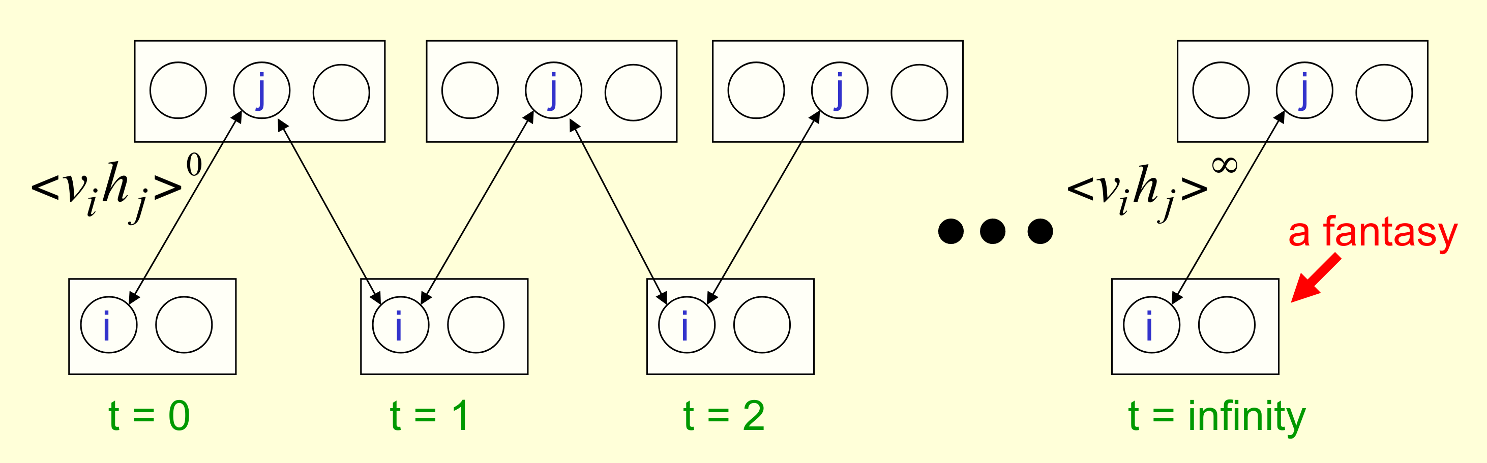
In 2012, I was in Austin sitting next to an ex-poker player named Amir who was singing Hinton’s praises. Hypnotized by his technicolor slides, I quit my job in a hurry and started an educational project using speech recognition and restricted Boltzmann machines. It never panned out, but I learned a lot about ASR and Android audio. Still love that idea.
In 2017, I started writing a book on the ethics of automation and predicted mass unemployment and social unrest. Although I got the causes wrong (pandemic, go figure), the information economy and confirmation bias takes were all dead right. Sadly, this is now driving the world completely insane. Don’t say I warned you, go out and fix our broken systems. The world needs more engineers who care.
In 2017, I witnessed the birth of differentiable programming, which I stole from Chris Olah and turned into a master’s thesis. Had a lot of trouble convincing people that classical programs could be made differentiable, but look at the proceedings of any machine learning conference today and you’ll find dozens of papers on differentiable sorting and rendering and simulation. Don’t thank me, thank Chris and the Theano guys.
In 2018, I correctly predicted Microsoft would acquire GitHub to mine code. Why MS and not Google? I’ll bet they tried, but Google’s leadership had fantasies of AGI and besides JetBrains, MS were the only ones who gave a damn about developers. Now ML4SE is a thriving research area and showing up in real products, much to the chagrin of those who believed ML was a fad. I suspect their hype filter blinded them to the value those tools provide.
Prediction: MS will acquire GH within five years. If the #ML4Code stuff delivers for MS, acquisition is highly likely. Although it would have been cheaper a few years ago. https://t.co/5ZMtiRtifD https://t.co/TaxkArm5ps
— breandan (@breandan) May 7, 2018

But to heck with everything I’ve said! If I had just one idea to share with these ML people, it would be types. Beat that drum as loud as I could. Types are the best tool we know for synthetic reasoning. If you want to build provably correct systems that scale on real-world applications, use types. Not everyone is convinced yet, but mark my words, types are coming. Whoever figures out how to connect types and learning will be the next Barbara Liskov or Frances Allen.
This year, I predicted the pandemic weeks before the lockdown, exited the market, and turned down a job at Google. Some people called me crazy. Now I’m going all-in on some new ideas (none of which are mine). I’m making some big bets and some will be wrong, but I see the very same spark of genius in them.
Everything old is new again
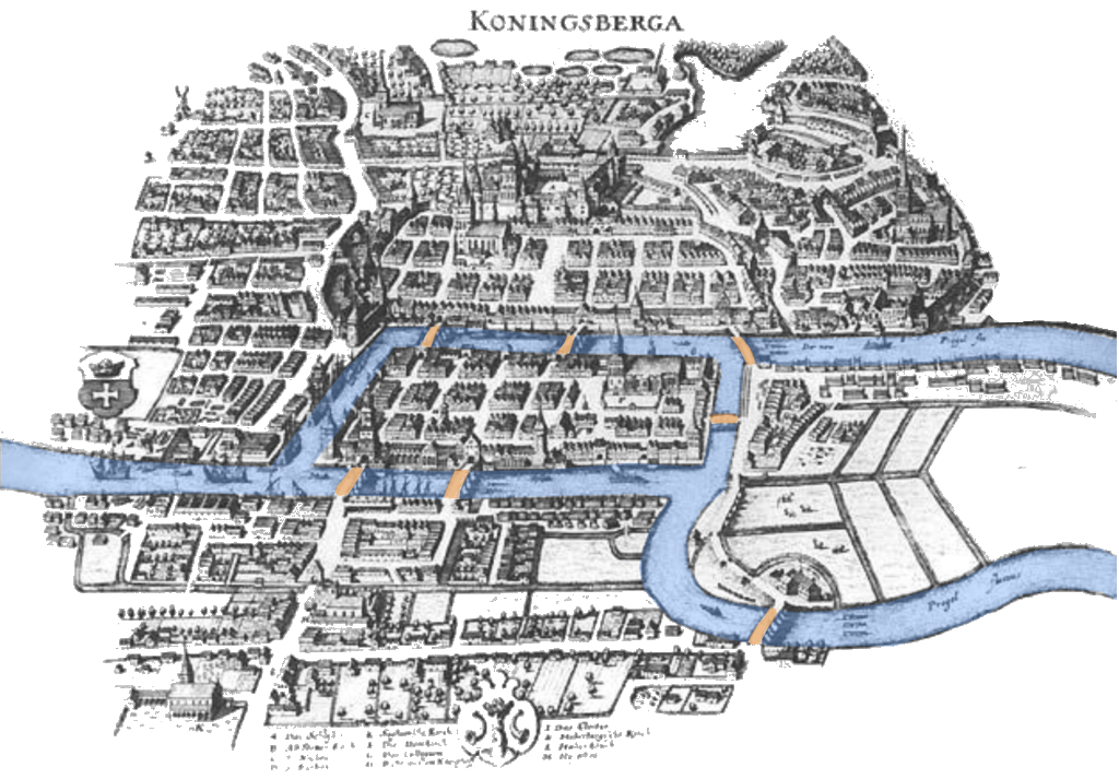
As a kid, I was given a book on the history of mathematics. I remember it had some interesting puzzles, including one with some bridges in a town divided by rivers, once inhabited by a man called Euler. Was there a tour crossing each bridge exactly once? Was it possible to tell without checking every path? I remember spending days trying to figure out the answer.
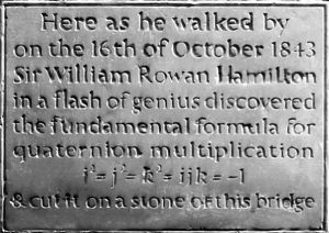
In the late 90s, my mom and I went to Ireland. I remember visiting Trinity College, and learning about a mathematician called Hamilton who discovered a famous formula connecting algebra and geometry, and carved it onto a bridge. We later visited the bridge, and the tour guide pointed out the stone, which we touched for good luck. The Irish have a thing for stones.
In 2007, I was applying to college and took the train from Boston to South Bend, Indiana, home of the Fighting Irish. Wandering about, I picked up a magazine article by a Hungarian mathematician called Barabási then at Notre Dame, who had some interesting things to say about complex networks. Later in 2009, while studying in Rochester, I carpooled with a nice professor, and learned complex networks are found in brains, languages and many marvelous places.
Fast forward to 2017. I was lured by the siren song of algorithmic differentiation. Olivier Breleux presented Myia and Buche. Matt Johnson gave a talk on Autograd. I met Chris Olah in Long Beach, who gave me the idea to study differentiable programming. I stole his idea, dressed it up in Kotlin and traded it for a POPL workshop paper and later a Master’s thesis. Our contributions were using algebra, shape inference and presenting AD as term rewriting.

In 2019, I joined a lab with a nice professor at McGill applying knowledge graphs to software engineering. Like logical reasoning, knowledge graphs are an idea from the first wave of AI in the 1960s and 70s which have been revived and studied in light of recent progress in the field. I believe this is an important area of research with a lot of potential. Knowledge and traceability plays a big role in software engineering, and it’s the bread-and-butter of a good IDE. The world needs better IDEs if we’re ever going to untangle this mess we’re in.
This Spring, I took a fascinating seminar on Graph Representation Learning. A lot of delightful graph theory has been worked out over the last decade. PageRank turned into power iteration. People have discovered many interesting connections to linear algebra, including Weisfeiler-Lehman graph kernels, graph Laplacians, Krylov methods, and spectral graph theory. These ideas have deepened our understanding of graph signal processing and its applications for learning and program analysis. More on that later.
What are graphs?
Graphs are general-purpose data structures used to represent a variety of data types and procedural phenomena. Unlike most sequential languages, graphs are capable of expressing a much richer family of relations between entities, and are a natural fit for many problems in computer science, physics, biology and mathematics. Consider the following hierarchy of data structures, all of which are graphs with increasing expressive power:
- Sets: datasets, multisets, posets, alphabets
- Sequences: Lists, strings, arrays, linear function composition
- Trees: Abstract syntax, XML, phylogeny, decision trees
- DAGs: Git, citations, dependency graphs, workflows, control flow, MLPs
- Directed graphs: State machines, λ-calculus, the web, call graphs, RNNs
- Hypergraphs: Knowledge, Zettelkasten, categories, physics, hypernetworks
As we realized in Kotlin∇, directed graphs can be used to model mathematical expressions, as well as other formal languages, including source code, intermediate representations and binary artifacts. Not only can graphs be used to describe extant human knowledge, many recent examples have shown that machines can “grow” trees and graphs for various applications, such as program synthesis, mathematical deduction and physical simulation. Recent neuro-symbolic applications have shown promising early results in graph synthesis:
- Learning to Represent Programs with Graphs, Allamanis et al., 2018
- Deep Learning for Symbolic Mathematics, Lample and Charton, 2019.
- Discovering Symbolic Models from Deep Learning with Inductive Biases, Cranmer et al., 2020.
- Symbolic Pregression: Discovering Physical Laws from Raw Distorted Video (Udrescu & Tegmark, 2020).
- DreamCoder: Growing generalizable, interpretable knowledge with wake-sleep Bayesian program learning, Ellis et al., 2020.
- Strong Generalization and Efficiency in Neural Programs, Li et al., 2020.
- Neural Execution of Graph Algorithms, Veličković et al. (2020)
The field of natural language processing has also developed a rich set of graph-based representations, such as constituency, dependency, link and other and other typed attribute grammars which can be used to reason about syntactic and semantic relations between natural language entities. Research has begun to show many practical applications for such grammars in the extraction and organization of human knowledge stored in large text corpora. Those graphs can be further processed into ontologies for logical reasoning.

Using coreference resolution and entity alignment techniques, we can reconstruct internally consistent relations between entities, which capture cross-corpus consensus in natural language datasets. When stored in knowledge graphs, these relations can be used for information retrieval and question answering, e.g. on wikis and other content management systems. Recent techniques have shown promise in automatic knowledge base construction (cf. Reddy et al., 2016).
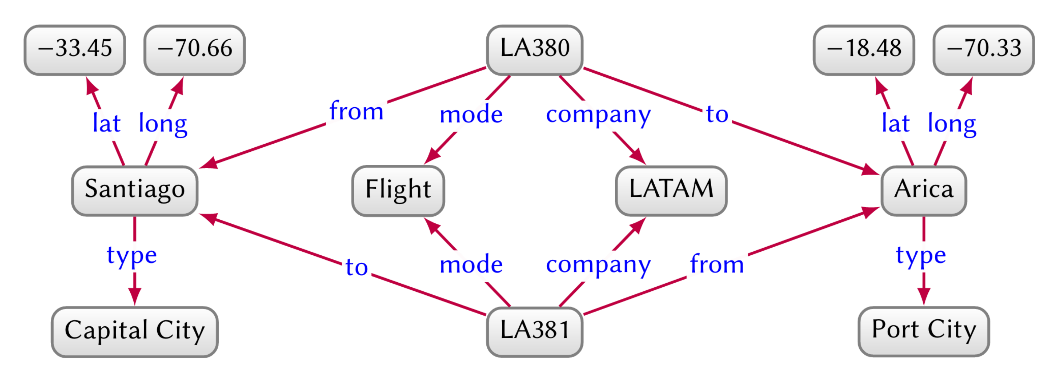
Lo and behold, the key idea behind knowledge graphs is our old friend, types. Knowledge graphs are multi-relational graphs whose nodes and edges possess a type. Two entities can be related by multiple types, and each type can relate many pairs of entities. We can index an entity based on its type for knowledge retrieval, and use types to reason about compound queries, e.g. “Which company has a direct flight from a port city to a capital city?”, which would otherwise be difficult to answer without a type system.
Induction introduction!
In this section, we will review some important concepts from Chomskyan linguistics, including finite automata, abstract rewriting systems, and λ-calculus. Readers already familiar with these concepts will gain a newfound appreciation for how each one shares a common thread and can be modeled using the same underlying abstractions.
Regular languages
One thing that always fascinated me is the idea of inductively defined languages, also known as recursive, or structural induction. Consider a very simple language that accepts strings of the form 0, 1, 100, 101, 1001, 1010, et cetera, but rejects 011, 110, 1011, or any string containing 11. The → symbol denotes a “production”. The | symbol, which we read as “or”, is just shorthand for defining multiple productions on a single line:
true → 1
term → 0 | 10 | ε
expr → term | expr term
We have two sets of productions, those which can be expanded, called “nonterminals”, and those which can be expanded no further, called “terminals”. Notice how each non-terminal occurs at most once in any single production. This property guarantees the language is recognizable by a special kind of graph, called a finite state machine. As their name suggests, FSMs contain a finite set of states, with labeled transitions between them:
| Finite Automaton | Library Courtesy Bell |
|---|---|
 |
 Please ring the bell once and wait for assistance. |
Imagine a library desk: you can wait quietly and eventually you will be served. Or, you can ring the bell once and wait quietly to be served. Should no one arrive after a while, you may press the bell again and continue waiting. Though you must never ring the bell twice, lest you disturb the patrons and be tossed out.
Regular languages can also model nested repetition. Consider a slightly more complicated language, given by the regular expression (0(01)*)*(10)*. The *, or Kleene star, means, “accept zero or more of the previous token”.
| | |
|
 |
Note here, a single symbol may have multiple transitions from the same state. Called a nondeterminsic finite automaton (NFA), this machine can occupy multiple states simultaneously. While no more powerful than their determinstic cousins, NFAs often require far fewer states to recognize the same language. One way to implement an NFA is to simulate the superposition of all states, by cloning the machine whenever such a transition occurs. More on that later.
Arithmetic
Now suppose we have a slightly more expressive language that accepts well-formed arithmetic expressions with up to two variables, in either infix or unary prefix form. In this language, a non-terminal may occur twice inside a single production – an expr can be composed of two subexprs:
term → 1 | 0 | x | y
  op → + | - | ·
expr → term | op expr | expr op expr
This is an example of a context-free language (CFL). We can represent strings in this language using a special kind of graph, called a syntax tree. Each time we expand an expr with a production rule, this generates a rooted subtree on op, whose branch(es) are exprs. Typically, syntax trees are inverted, with branches extending downwards, like so:
| Syntax Tree | Peach Tree |
|---|---|
 |
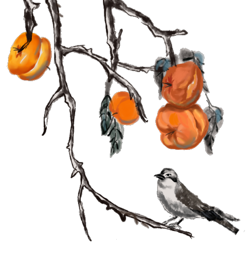 |
While syntax trees can be interpreted computationally, they do not actually perform computation unless evaluated. To [partially] evaluate a syntax tree, we will now introduce some pattern matching rules. Instead of just allowing terminals to occur on the right-hand side of a production, suppose we also allow terminals on the left, and applying a rule can shrink a string in our language. Here, we use capital letters on the same line to indicate an exact match, e.g. a rule U + V → V + U would replace x + y with y + x:
                                         E + E → +E
                                         E · E → ·E
                  E + 1 | 1 + E | +1 | -0 | ·1 → 1
                         E + 0 | 0 + E | E - 0 → E
  E - E | E · 0 | 0 · E | 0 - E | +0 | -1 | ·0 → 0
If we must add two identical expressions, why evaluate them twice? If we need to multiply an expression by 0, why evaluate it at all? Instead, we will try to simplify these patterns whenever we encounter them. This is known as a rewrite system, which we can think of as grafting or pruning the branches of a tree. Some say, “all trees are DAGs, but not all DAGs are trees”. I prefer to think of a DAG as a tree with a gemel:
| Rewrite Rule | Deformed Tree |
|---|---|
 |
 |
 |
 |
Let us now introduce a new operator, Dₓ, and some corresponding rules. In effect, these rules will push Dₓ as far towards the leaves as possible, while rewriting terms along the way. We will also introduce some terminal rewrites:
[R0]       term → Dₓ(term)
[R1]      Dₓ(x) → 1
[R2]      Dₓ(y) → 0
[R3]    Dₓ(U+V) → Dₓ(U) + Dₓ(V)
[R4]    Dₓ(U·V) → U·Dₓ(V) + Dₓ(U)·V
[R5]     Dₓ(+U) → +Dₓ(U)
[R6]     Dₓ(-U) → -Dₓ(U)
[R7]     Dₓ(·U) → +U·Dₓ(U)
[R8]      Dₓ(1) → 0
[R9]      Dₓ(0) → 0
Although we assign an ordering R0-R9 for notational convenience, an initial string, once given to this system, will always converge to the same result, no matter in which order we perform the substitutions (proof required):
| Term Confluence | Ottawa-St. Lawrence Confluence |
|---|---|
 |
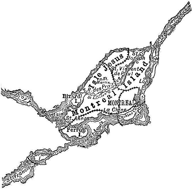 |
This feature, called confluence, is an important property of some rewrite systems: regardless of the substitution order, we will eventually arrive at the same result. If all strings in a language reduce to a form which can be simplified no further, we call such systems strongly normalizing, or terminating. If a rewriting system is both confluent and terminating it is said to be convergent.
λ-calculus
So far, the languages we have seen are capable of generating and simplifying arithmetic expressions, but are by themselves incapable of performing arithmetic, since they cannot evaluate arbitrary arithmetic expressions. We will now consider a language which can encode and evaluate any arithmetic expression:
expr → var | func | appl
func → (λ var.expr)
appl → (expr expr)
To evaluate an expr in this language, we need a single substitution rule. The notation expr[var → val], we read as, “within expr, var becomes val”:
(λ var.expr) val → (expr[var → val])
For example, applying the above rule to the expression (λy.y z) a yields a z. With this seemingly trivial addition, our language is now powerful enough to encode any computable function! Known as the pure untyped λ-calculus, this system is equivalent to an idealized computer with infinite memory.
While grammatically compact, computation in the λ-calculus is not particularly terse. In order to perform any computation, we will need a way to encode values. For example, we can encode the boolean algebra like so:
[D1]           λx.λy.x = T     "true"
[D2]           λx.λy.y = F     "false"
[D3]       λp.λq.p q p = &     "and"
[D4]       λp.λq.p p q = |     "or"
[D5]    λp.λa.λb.p b a = !     "not"
To evaluate a boolean expression !T, we will first need to encode it as a λ-expression. We can then evaluate it using the λ-calculus as follows:
  (           !          ) T
→ (λp.λa.λb.    p     b a) T   [D5]
→ (   λa.λb.    T     b a)     [p → T]
→ (   λa.λb.(λx.λy.x) b a)     [D1]
→ (   λa.λb.(   λy.b)   a)     [x → b]
→ (   λa.λb.(   λy.b)    )     [y → a]
→ (   λa.λb.b            )     [y →  ]
→ (   F                  )     [D2]
We have reached a terminal, and can recurse no further. This particular program is decidable. What about others? Let us consider an undecidable example:
(λg.(λx.g (x x)) (λx.g (x x))) f
    (λx.f (x x)) (λx.f (x x))                        [g → f]
        f (λx.f (x x))(λx.f (x x))                   [f → λx.f(x x)]
        f     f (λx.f (x x))(λx.f (x x))             [f → λx.f(x x)]
        f     f     f (λx.f (x x))(λx.f (x x))       [f → λx.f(x x)]
        ...                 (λx.f (x x))(λx.f (x x)) [f → λx.f(x x)]
This pattern is Curry’s (1930) famous fixed point combinator and the cornerstone of recursion, called Y. Unlike its typed cousin, the untyped λ-calculus is not strongly normalizing and thus not guaranteed to converge. Were it convergent, it would not be Turing-complete. This hard choice between decidability and universality is one which no computational language can avoid.
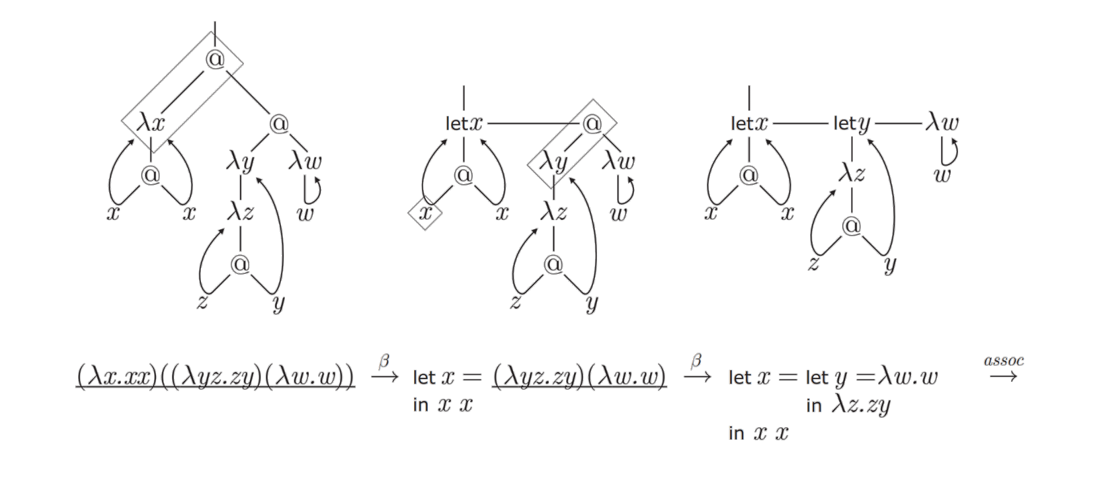
The λ-calculus, can also be interpreted graphically. I refer the curious reader to some promising proposals which have attempted to formalize this perspective:
- An Algorithm for Optimal Lambda Calculus Reduction, (Lample 1990)
- A Graphical Notation for the Lambda Calculus (Keenan, 1996)
- Visual lambda calculus (Massalõgin, 2008)
- Graphic lambda calculus (Buliga, 2013)
- Lambda Diagrams (Tromp, 2014)
Cellular automata
The elementary cellular automaton is another string rewrite system consisting of a one dimensional binary array, and a 3-cell grammar. Note there are \(2^{2^3} = 256\) possible rules for rewriting the tape. It turns out even in this tiny space, there exist remarkable automata. Consider the following rewrite system:
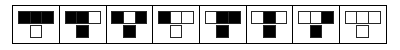
| current pattern | 111 |
110 |
101 |
100 |
011 |
010 |
001 |
000 |
|---|---|---|---|---|---|---|---|---|
| next pattern | ` 0 ` | ` 1 ` | ` 1 ` | ` 0 ` | ` 1 ` | ` 1 ` | ` 1 ` | ` 0 ` |
We can think of this machine as sliding over the tape, and replacing the centermost cell in each matching substring with the second value. Depending on the initial state and rewrite pattern, cellular autoamta can produce many visually interesting patterns. Some have spent a great deal of effort cataloguing families of CA and their behavior. Following Robinson (1987), we can also define an ECA inductively, using the following recurrence relation:
\[a_i^{(t)} = \sum_j s(j)a_{(i-j)}^{t-1} \mod m\]This characterization might remind us of a certain operation from digital signal processing, called a discrete convolution. We read \(f * g\) as “\(f\) convolved by \(g\)”:
\[(f * g)[n] = \sum_m f[m]g[n-m]\]Here \(f\) is our state and \(g\) is called a “kernel”. Similar to the λ-calculus, this language also is known to be universal. Disregarding efficiency, we could encode any computable function as an initial state and mechanically apply Rule 110 to simulate a TM, λ-calculus, or any other TC system for that matter.
Cellular automata can also be interpreted as a graph rewriting system, although the benefits of this perspective are not as clear. Unlike string rewriting, graph substitution is much more difficult to implement efficiently, as pattern matching amounts to subgraph isomorphism, which is NP-complete. While there are some optimizations to mitigate this problem, graph grammars do not appear to confer any additional computational benefits. Nevertheless, it is conceptually interesting.
Graphs, inductively
Just like grammars, we can define graphs themselves inductively. As many graph algorithms are recursive, this choice considerably simplifies their implementation. Take one definition of an unlabeled directed graph, proposed by Erwig (2001). Here, the notation list → [item] is shorthand for list → item list, where item is some terminal, and list is just a list of items:
vertex  → int
adj     → [vertex]
context → (adj, vertex, adj)
graph   → empty | context & graph
Erwig defines a graph in four parts. First, we have a vertex, which is simply an integer. Next we have a list of vertices, adj, called an adjacency list. The context is a 3-tuple containing a vertex and symmetric references to its inbound and outbound neighbors, respectively. Finally, we have the inductive case: a graph is either (1) empty, or (2) a context and a graph.
| | |
|
 |
Let us consider a directed graph implementation in Kotlin. We do not store inbound neighbors, and attempt to define a vertex as a closed neighborhood:
open class Graph(val vertices: Set<Vertex>) { ... }
data class Vertex(neighbors: Set<Vertex>): Graph(this + neighbors)
//                                               ↳ Compile error!
Note the coinductive definition, which creates problems right off the bat. Since this is not accessible inside the constructor, we cannot have cycles or closed neighborhoods, unless we delay edge instantiation until after construction:
class Graph(val vertices: Set<Vertex>) { ... }
class Vertex(adjacencyMap: (Vertex) -> Set<Vertex>) {
  constructor(neighbors: Set<Vertex> = setOf()) : this({ neighbors })
  val neighbors = adjacencyMap(this).toSet()
}
We can now call Vertex() { setOf(it) } to create loops and closed neighborhoods. This definition admits a nice k-nearest neighbors implementation, allowing us to compute the k-hop transitive closure of a vertex or set of vertices:
tailrec fun Vertex.neighbors(k: Int = 0, vertices: Set<Vertex> =
                             neighbors + this): Set<Vertex> =
  if (k == 0 || vertices.neighbors() == vertices) vertices
  else knn(k - 1, vertices + vertices.neighbors() + this)

fun Set<Vertex>.neighbors() = flatMap { it.neighbors() }.toSet()

// Removes all vertices outside the set
fun Set<Vertex>.closure(): Set<Vertex> =
  map { vertex -> Vertex(neighbors.filter { it in this }) }.toSet()

fun Vertex.neighborhood(k: Int = 0) = Graph(neighbors(k).closure())
Another useful representation for a graph, which we will describe in further detail below, is a matrix. We can define the adjacency, degree, and Laplacian matrices like so:
val Graph.adjacency = Mat(vertices.size, vertices.size).also { adj ->
  vertices.forEach { v -> v.neighbors.forEach { n -> adj[v, n] = 1 } }
}

val Graph.degree = Mat(vertices.size, vertices.size).also { deg ->
  vertices.forEach { v -> deg[v, v] = v.neighbors.size }
}

val Graph.laplacian = degree - adjacency
These matrices have some important applications in algebraic and spectral graph theory, which we will have more to stay about later.
Weisfeiler-Lehman
Let us consider an algorithm called the Weisfeiler-Lehman isomorphism test, on which my colleague David Bieber has written a nice piece. I’ll focus on its implementation. First, we need a pooling operator, which will aggregate all neighbors in a node’s neighborhood using some summary statistic:
fun Graph.poolBy(statistic: Set<Vertex>.() -> Int): Map<Vertex, Int> =
  nodes.map { it to statistic(it.neighbors()) }.toMap()
Next, we’ll define a histogram, which just counts each node’s neighborhood:
val Graph.histogram: Map<Vertex, Int> = poolBy { size }
Now we’re ready to define the Weisfeiler-Lehman operator, which recursively hashes the labels until fixpoint termination:
tailrec fun Graph.wl(labels: Map<Vertex, Int>): Map<Vertex, Int> {
  val next = poolBy { map { labels[it]!! }.sorted().hash() }
  return if (labels == next) labels else wl(next)
}
With one round, we’re just comparing the degree histogram. We compute the hash of the entire graph by hashing the multiset of WL labels:
fun Graph.hash() = wl(histogram).values.sorted().hash()
Finally, we can define a test to detect if one graph is isomorphic to another:
fun Graph.isIsomorphicTo(that: Graph) =
  this.nodes.size == that.nodes.size &&
  this.numOfEdges == that.numOfEdges &&
  this.hash() == that.hash()
This algorithm works on many graphs encountered in the wild, however it cannot distinguish two regular graphs with an identical number of vertices and edges. Nevertheless, it is appealing for its simplicity and exemplifies a simple “message passing” algorithm, which we will revisit later. For a complete implementation and other inductive graph algorithms, such as Barabási’s preferential attachment algorithm, check out Kaliningraph.
Graph Diameter
A graph’s diameter is the length of the longest shortest path between any two of its vertices. Let us define the augmented adjacency matrix as \(A + A^\intercal + \mathbb{1}\), or:
val Graph.A_AUG = adjacency.let { it + it.transpose() } + ONES
To compute the diameter of a connected graph \(G\), we can simply power the augmented adjacency matrix until it contains no zeros:
/* (A')ⁿ[a, b] counts the number of walks between vertices a, b of
 * length n. Let i be the smallest natural number such that (A')ⁱ
 * has no zeros. i is the length of the longest shortest path in G.
 */

tailrec fun Graph.slowDiameter(i: Int = 1, walks: Mat = A_AUG): Int =
  if (walks.data.all { 0 < it }) i
  else slowDiameter(i = i + 1, walks = walks * A_AUG)
If we consider the complexity of this procedure, we note it takes \(\mathcal O(M \mid G\mid)\) time, where \(M\) is the complexity of matrix multiplication, and \(\mathcal O(Q\mid G \mid^2)\) space, where \(Q\) is the number of bits required for a single entry in A_AUG. Since we only care whether or not the entries are zero, we can instead cast A_AUG to \(\mathbb B^{n\times n}\) and run binary search for the smallest i yielding a matrix with no zeros:
tailrec fun Graph.fastDiameter(i: Int = 1,
    prev: Mat = A_AUG, next: Mat = prev): Int =
  if (next.isFull) slowDiameter(i / 2, prev)
  else fastDiameter(i = 2 * i, prev = next, next = next * next)
Our improved procedure fastDiameter runs in \(\mathcal O(M\log_2\mid G\mid)\) time. An iterative version of this procedure may be found in Booth and Lipton (1981).
Graph Neural Networks
A graph neural network is like a graph, but whose edges are neural networks. In its simplest form, the inference step can be defined as a matrix recurrence relation \(\mathbf H^t := σ(\mathbf A \mathbf H^{t-1} \mathbf W^t + \mathbf H^{t-1} \mathbf W^t)\) following Hamilton (2020):
tailrec fun gnn(
  // Number of message passing rounds
  t: Int = fastDiameter(),
  // Matrix of node representations ℝ^{|V|xd}
  H: Mat,
  // (Trainable) weight matrix ℝ^{dxd}
  W: Mat = randomMatrix(H.numCols),
  // Bias term ℝ^{dxd}
  b: Mat = randomMatrix(size, H.numCols),
  // Nonlinearity ℝ^{*} -> ℝ^{*}
  σ: (Mat) -> Mat = { it.elwise { tanh(it) } },
  // Layer normalization ℝ^{*} -> ℝ^{*}
  z: (Mat) -> Mat = { it.meanNorm() },
  // Message ℝ^{*} -> ℝ^{*}
  m: Graph<G, E, V>.(Mat) -> Mat = { σ(z(A * it * W + it * W + b)) }
): Mat = if(t == 0) H else gnn(t = t - 1, H = m(H), W = W, b = b)
The important thing to note here is that this message passing procedure is a recurrence relation, which like the graph grammar and WL algorithm seen earlier, can be defined inductively. Hamilton et al. (2017) also consider induction in the context of representation learning, although their definition is more closely related to the concept of generalization. It would be interesting to explore the connection between induction in these two settings, and we will have more to say about matrix recurrence relations in a bit.
Graph languages
Approximately 20% of the human cerebral cortex is devoted to visual processing. By using visual representations, language designers can tap into powerful pattern matching abilities which are often underutilized by linear symbolic writing systems. Graphs are one such example which have found many applications as reasoning and communication devices in various domain-specific languages:
| Language | Example |
|---|---|
| Finite automata |  |
| Tensor networks | 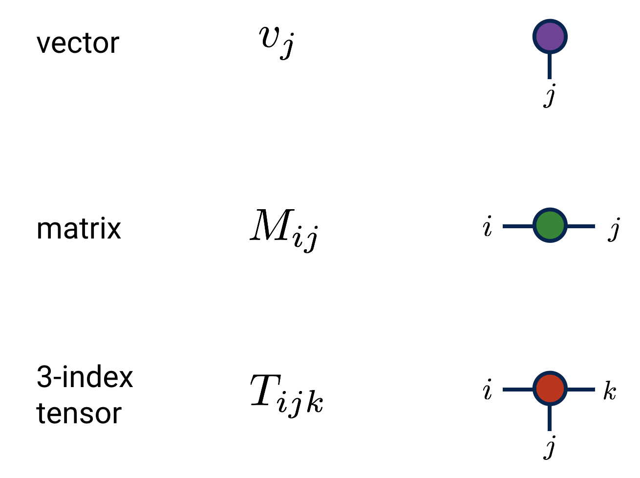 |
| Causal graphs |  |
| Category theory |  |
| Penrose notation |  |
| Feynman diagrams |  |
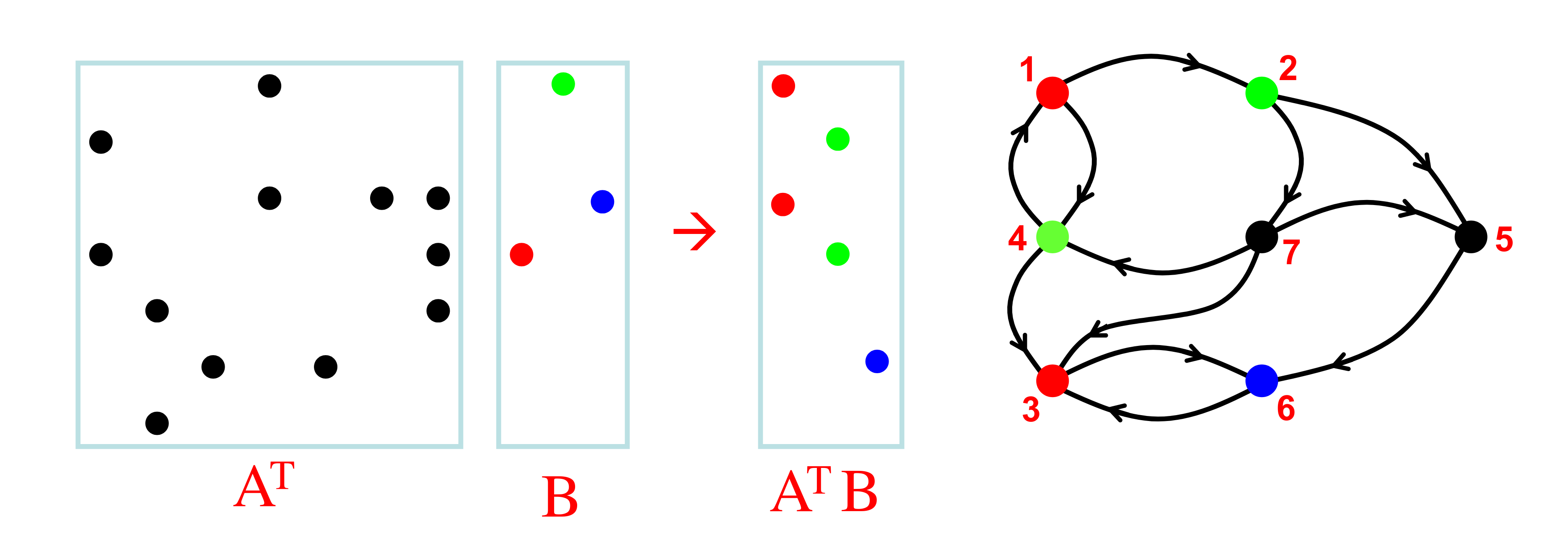
As Bradley (2019) vividly portrays in her writing, we can think of a matrix as not just a two-dimensional array, but a function on a vector space. This perspective can be depicted using a bipartite graph:
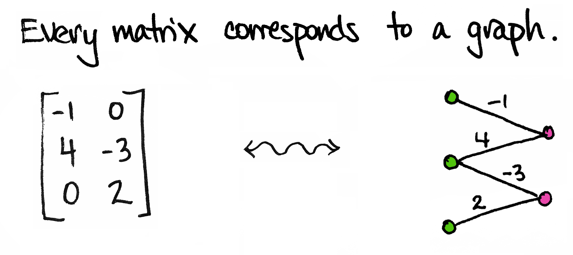
Not only do matrices correspond to graphs, graphs also correspond to matrices. One way to think of a graph is just a boolean matrix, or real matrix for weighted graphs. Consider an adjacency matrix containing nodes V, and edges E, where:
\[\begin{align*} \mathbf A \in \mathbb B^{|V|\times|V|} \text{ where } \mathbf A[u, v] = \begin{cases} 1,& \text{if } u, v \in E \\ 0,& \text{otherwise} \end{cases} \end{align*}\]| | |
 |
 |
Note the lower triangular structure of the adjacency matrix, indicating it contains no cycles, a property that is not immediately obvious from the naïve geometric layout. Any graph whose adjacency matrix can be reordered into triangular form is a directed acyclic graph. Called a topological ordering, this algorithm can be implemented by repeatedly squaring the adjacency matrix.
Both the geometric and matrix representations impose an extrinsic perspective on graphs, each with their own advantages and drawbacks. 2D renderings can be visually compelling, but require solving a minimal crossing number or similar optimization to make connectivity plain to the naked eye. While graph drawing is an active field of research, matrices can often reveal symmetries that are not obvious from a naïve graph layout (and vis versa).
Matrices are problematic for some reasons. Primarily, by treating a graph as a matrix, we impose an ordering over all vertices which is often arbitrary. Note also its sparsity, and consider the size of the matrix required to store even small graphs. While problematic, this can be overcome with certain optimizations. Despite these issues, matrices and are a natural representation choice for many graph algorithms, particularly on modern parallel processing hardware.
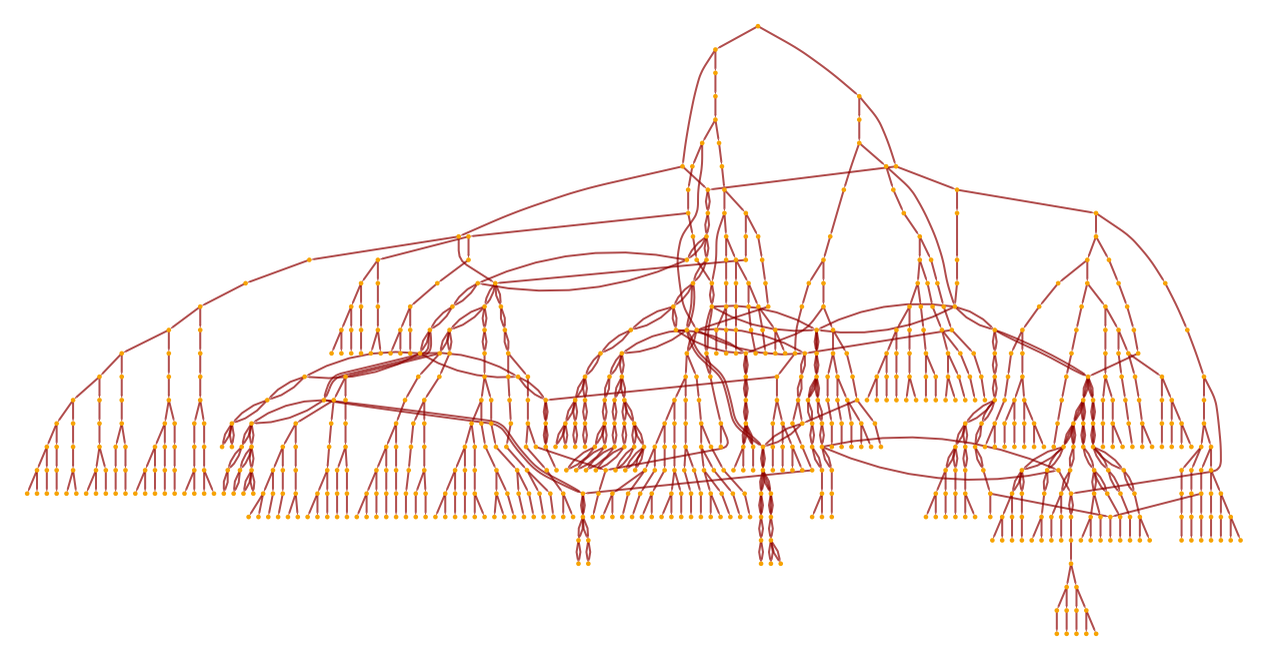
Just like matrices, we can also think of a graph as a function, or transition system, which carries information from one state to the next - given a state or set of states, the graph tells us which other states are reachable. Recent work in graph theory has revealed a fascinating duality between graphs and linear algebra, holding many important insights for dynamical processes on graphs.
Graphs, computationally
What happens when we take a square matrix \(\mathbb{R}^{n\times n}\) and raise it to a power? Which kinds of matrices converge and what are their asymptotics? This is a very fertile line of inquiry which has occupied engineers for the better part of the last century, with important applications in statistical phyics, control theory, and deep learning. Linear algebra gives us many tricks for designing the matrix and normalizing the product to promote convergence.
One way to interpret this is as follows: each time we multiply a matrix by a vector \(\mathbb{R}^{n}\), we are effectively simulating a dynamical system at discrete time steps. This method is known as power iteration or the Krylov method in linear algebra. In the limit, we are seeking fixpoints, or eigenvectors, which are these islands of stability in our dynamical system. If we initialize our state at such a point, the transition matrix will send us straight back to where we started.
\[f(x, y) = \begin{bmatrix} \frac{cos(x+2y)}{x} & 0 \\ 0 & \frac{sin(x-2y)}{y} \end{bmatrix} * \begin{bmatrix}x\\y\end{bmatrix} = \begin{bmatrix}cos(x+2y)\\sin(x-2y)\end{bmatrix}\]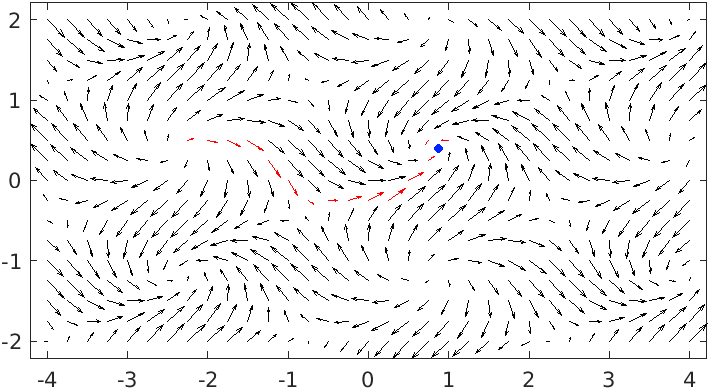
Locating a point where \(f(x, y) = f\circ f(x, y)\), indicates the trajectory has terminated. There exists a famous theorem from Brouwer: given a set \(S\) which contains its limits (i.e. closed), whose contents are all a finite distance apart (i.e. bounded), every continuous function from the set onto itself (\(f: S \rightarrow S\)) will map at least one of its members \(x: S\), called a fixpoint, onto itself (\(f(x)=x\)). Such points describe the asymptotic behavior of our function.
First, let’s get some definitions out of the way.
  𝔹 → True | False
  𝔻 → 1 | ... | 9
  ℕ → 𝔻 | 𝔻0  | 𝔻ℕ
  ℤ → 0 | ℕ   | -ℕ
  ℚ → ℕ | ℤ/ℕ
  ℝ → ℕ | ℕ.ℕ | -ℝ
  ℂ → ℝ + ℝi
  ℍ → ℝ + ℝi + ℝj + ℝk
  T → 𝔹 | ℕ | ℤ | ℚ | ℝ | ℂ | ℍ
  n → ℕ
vec → [Tⁿ]
mat → [[Tⁿ]ⁿ]
We can think of the Krylov method as either a matrix-matrix or matrix-vector product, or a recurrence relation with some normalization:
Krylov Method
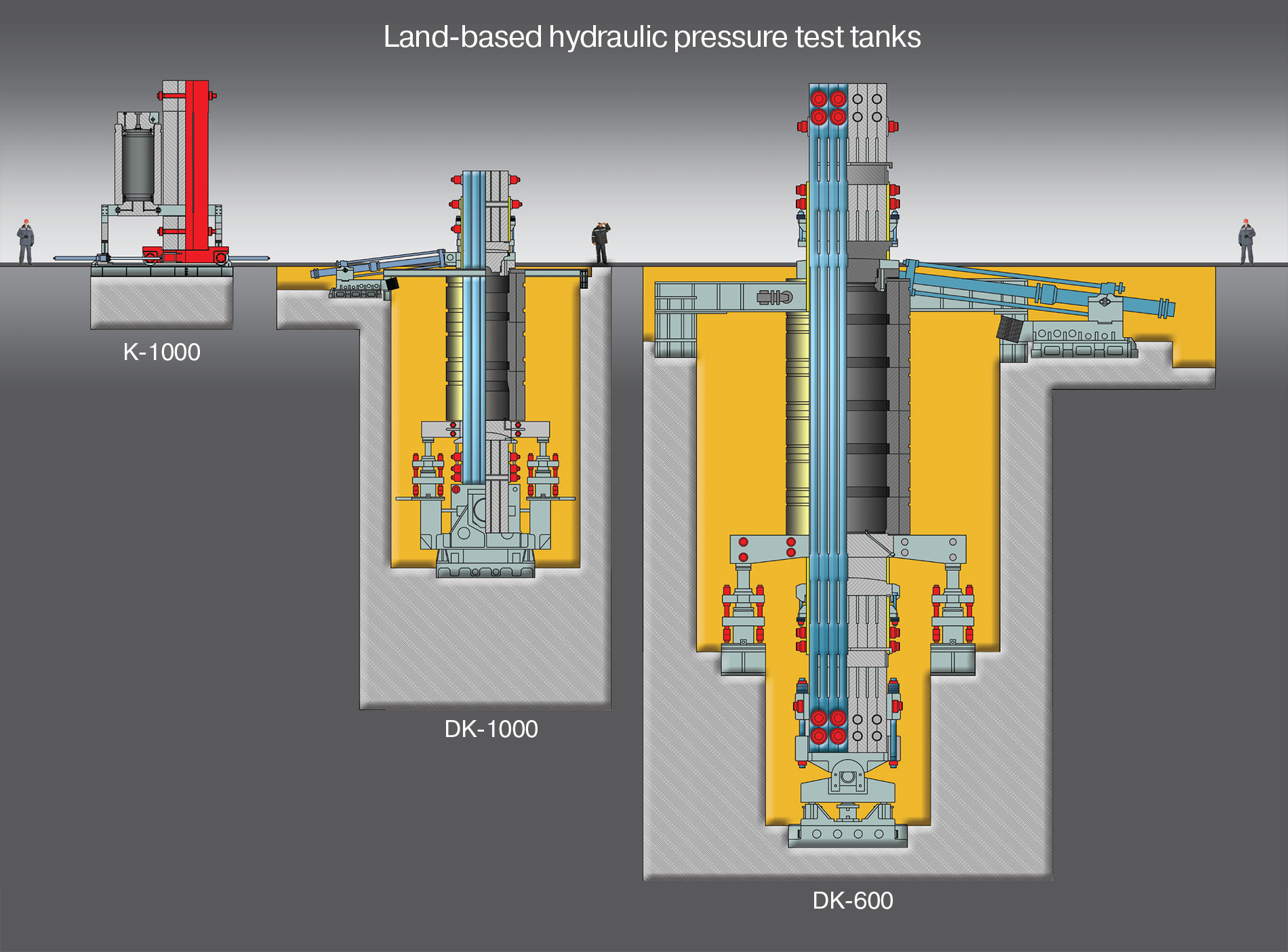
There exists in St. Petersburg a naval research facility, known as the Krylov Shipbuilding Research Institute, which houses the world's largest full ocean depth hydraulic pressure tank. Capable of simulating in excess of 20,000 PSI, the DK-1000 is used to test deepwater submersible vessels. At such pressure, even water itself undergoes ~5% compression. Before inserting your personal submarine, you may wish to perform a finite element analysis to check hull integrity. Instabilities in the stiffness matrix may produce disappointing results.

| | |
|
\((\mathbf{M}\mathbf{M})\mathbf{v}, (\mathbf{M}\mathbf{M}\mathbf{M})\mathbf{v}, \ldots\) |
|
\(\mathbf{M}(\mathbf{M}\mathbf{v}), \mathbf{M}(\mathbf{M}(\mathbf{M}\mathbf{v})), \ldots\) |
|
\(\frac{\mathbf{M}\mathbf{v}}{\|\mathbf{M}\mathbf{v}\|}, \frac{\mathbf{M}\frac{\mathbf{M}\mathbf{v}}{\|\mathbf{M}\mathbf{v}\|}}{\|\mathbf{M}\frac{\mathbf{M}\mathbf{v}}{\|\mathbf{M}\mathbf{v}\|}\|}, \frac{\mathbf{M}\frac{\mathbf{M}\frac{\mathbf{M}\mathbf{v}}{\|\mathbf{M}\mathbf{v}\|}}{\|\mathbf{M}\frac{\mathbf{M}\mathbf{v}}{\|\mathbf{M}\mathbf{v}\|}\|}}{\|\mathbf{M}\frac{\mathbf{M}\frac{\mathbf{M}\mathbf{v}}{\|\mathbf{M}\mathbf{v}\|}}{\|\mathbf{M}\frac{\mathbf{M}\mathbf{v}}{\|\mathbf{M}\mathbf{v}\|}\|}\|}, \ldots\) |
Regrouping the order of matrix multiplication offers various computational benefits, and adding normalization prevents singularities from emerging. Alternate normalization schemes have been developed for various applications in graphs. This sequence forms the so-called Krylov matrix (Krylov, 1931):
\[\mathbf{K}_{i} = \begin{bmatrix}\mathbf{v} & \mathbf{M}\mathbf{v} & \mathbf{M}^{2}\mathbf{v} & \cdots & \mathbf{M}^{i-1}\mathbf{v} \end{bmatrix}\]There exists a famous theorem known as the Perron-Frobenius theorem, which states that if \(\mathbf M \in \mathcal T^{n \times n}\), then \(\mathbf M\) has a unique largest eigenvalue \(\lambda \in \mathcal T\) and dominant eigenvector \(\mathbf{q} \in \mathcal T^{n}\). It has long been known that under some weak assumptions, \(\lim_{i\rightarrow \infty} \mathbf{M}^i \mathbf{v} = c\mathbf{q}\) where \(c\) is some constant. We are primarily interested in determinstic transition systems, where \(\mathcal T \in \{\mathbb B, \mathbb N\}\).
The Krylov methods have important applications for studying dynamical systems and graph signal processing. Researchers are just beginning to understand how eigenvalues of the graph Laplacian affect the asymptotics of dynamical processes on graphs. We have already seen one example of these in the WL algorithm. Another example of graph computation can be found in Valiant (1975), who shows a CFL parsing algorithm which is equivalent to matrix multiplication.
TIL: CFL parsing can be reduced to boolean matrix multiplication (Valiant, 1975), known to be subcubic (Strassen, 1969), and later proven an asymptotic lower bound (Lee, 1997). This admits efficient GPGPU implementation (Azimov, 2017) in @YaccConstructor https://t.co/3Vbml0v6b9
— breandan (@breandan) June 28, 2020
Yet another example of graph computation can be found in Reps et al. (2016), who show that boolean matrix algebra can be used for abstract interpretation. By representing control flow graphs as boolean matrix expressions, they show how to apply root-finding techniques like Newton’s method (first observed by Esparza et al. (2010)) to dataflow analysis, e.g. for determining which states are reachable from some starting configuration by computing their transitive closure:
Newton's method has some amazing applications for program analysis. Reps et al. (2016) show a mapping between control flow graphs and boolean matrix expressions. Graph reachability amounts to finding fixed points of a semiring equation. What a goldmine! https://t.co/BFCZiJ1b6n pic.twitter.com/Jd86bEXiIu
— breandan (@breandan) July 12, 2020
We could spend all day listing various matrix algorithms for graph computation. Certainly, far better writers have done them justice. Instead, let’s just give some simple examples of dynamical processes on graphs.
Examples
What happens if we define arithmetic operations on graphs? How could we define these operations in a way that allows us to perform computation? As we already saw, one way to represent a directed graph is just a square matrix whose non-zero entries indicate edges between nodes. Just like real matrices in linear algebra, we can add, subtract, multiply and exponentiate them. Other composable operations are also possible.
We will now show a few examples simulating a state machine using the Krylov method. For illustrative purposes, the state simply holds a vector of binary or integer values, although we can imagine it carrying other “messages” around the graph in a similar manner, using another algebra. Here, we will use the boolean algebra for matrix multiplication, where + corresponds to logical disjunction (∨), and * corresponds to logical conjunction (∧):
┌───┬───┬─────┬─────┐
│ x │ y │ x*y │ x+y │        Boolean Matrix Multiplication
├───┼───┼─────┼─────┤ ┌─       ─┐ ┌─ ─┐ ┌─                     ─┐
│ 0 │ 0 │  0  │  0  │ │ a  b  c │ │ j │ │ a * j + b * k + c * l │
│ 0 │ 1 │  0  │  1  │ │ d  e  f │*│ k │=│ d * j + e * k + f * l │
│ 1 │ 0 │  0  │  1  │ │ g  h  i │ │ l │ │ g * j + h * k + i * l │
│ 1 │ 1 │  1  │  1  │ └─       ─┘ └─ ─┘ └─                     ─┘
└───┴───┴─────┴─────┘
Linear chains
Let’s iterate through a linked list. To do so, we will initialize the pointer to the head of the list, and use multiplication to advance the pointer by a single element. We add an implicit self-loop to the final node, and halt whenever a fixpoint is detected. This structure is known as an absorbing Markov chain.
 |
|
|
|
 |
|
|
|
 |
|
|
|
Nondeterminstic finite automata
Simulating a DFA using a matrix can be inefficient since we only ever inhabit one state at a time. The real benefit of using matrices comes when simulating nondeterminstic finite automata, seen earlier.
Formally, an NFA is a 5-tuple \(\langle Q, \Sigma, \Delta, q_0, F \rangle\), where \(Q\) is a finite set of states, \(\Sigma\) is the alphabet, \(\Delta :Q\times (\Sigma \cup \{\epsilon \})\rightarrow P(Q)\) is the transition function, \(q_0 \in Q\) is the initial state and \(F \subseteq Q\) are the terminal states. An NFA can be represented as a labeled transition system, or directed graph whose adjacency matrix is defined by the transition function, with edge labels representing symbols from the alphabet and self-loops for each terminal state, both omitted for brevity.
Typical implementations often require cloning the NFA when multiple transitions are valid, which can be inefficient. Instead of cloning the machine, we can simulate the superposition of all states using a single data structure:
 |
|
|
|
 |
|
|
|
 |
|
|
|
We encode the accept state as a self cycle in order to detect the fixpoint criterion \(S_{t+1} = S_{t}\), after which we halt execution.
Dataflow graphs
Suppose we have the function f(a, b) = (a + b) * b and want to evaluate f(2, 3). For operators, we will need two tricks. First, all operators will retain their state, i.e. 1s along all operator diagonals. Second, when applying the operator, we will combine values using the operator instead of performing a sum.
 |
|
|
|
 |
|
|
|
 |
|
|
|
Did you know? Arithmetic expressions can be efficiently parallelized using matrix arithmetic (Miller et al., 1987): https://t.co/9Tr9hImPFA pic.twitter.com/8vBv9phssk
— breandan (@breandan) July 15, 2020
The author was very excited to discover this technique while playing with matrices one day, only later to discover it was described 33 years earlier by Miller et al. (1987). Miller was inspired by Valiant et al.’s (1983) work in arithmetic circuit complexity, who was in turn inspired by Borodin et al.’s (1982) work on matrix computation. This line of research has recently been revisited by Nisan and Wigderson (1997) and later Klivans and Shpilka (2003) which seeks to understand how circuit size and depth affects learning complexity.
Graphs, efficiently
Due to their well-studied algebraic properties, graphs are suitable data structures for a wide variety of applications. Finding a reduction to a known graph problem can save years of effort, but graph algorithms can be challenging to implement efficiently, as dozens of libraries and compiler frameworks have found. Why have efficient implementations proven so difficult, and what has changed?
One issue hindering efficient graph representation is their space complexity. Suppose we have a graph with \(10^5=100,000\) nodes, but only a single edge. We will need \(10^{5\times 2}\) bits, or about 1 GB to store its adjacency matrix, where an equivalent adjacency list would only consume \(\lceil 2\log_2 10^5 \rceil = 34\) bits. Most graphs are similarly sparse. But how do you multiply adjacency lists? One solution is to use a sparse matrix, which is spatially denser proportional to its sparsity and can be linearly faster on parallel computing architectures.
Perhaps the more significant barrier to widespread adoption of graph algorithms is their time complexity. Many interesting problems on graphs are NP-complete, including Hamiltonian path detection, TSP and subgraph isomorphism. Many of those problems have approximations which are often tolerable, but even if exact solutions are needed, CS theory is primarily concerned with worst-case complexity, which seldom or rarely occurs in practice. Natural instances can often be solved quickly using heuristic-guided search, such as SAT or SMT solvers.
Most graph algorithms are currently implemented using object oriented or algebraic data types as we saw previously. While conceptually simple to grasp, this approach is computationally inefficient. We would instead prefer a high level API backed by a pure BLAS implementation. As numerous papers have shown, finding an efficient matrix representation opens the path to optimized execution on GPUs or SIMD-capable hardware. For example, all of the following automata can be greatly accelerated using sparse matrix arithmetic on modern hardware:
Suppose we want to access the source code of a program from within the program itself. How could we accomplish that? There is a famous theorem by Kleene which gives us a clue how to construct a self-replicating program. More specifically, we need an intermediate representation, or reified computation graph (i.e. runtime-accessible IR). Given any variable y, we need some method y.graph() which programmatically returns its transitive closure, including upstream dependencies and downstream dependents. Depending on scope and granularity, this graph can expand very quickly, so efficiency is key.

With the advent of staged metaprogramming in domain-specific languages like TensorFlow and MetaOCaml, such graphs are available to introspect at runtime. By tracing all operations (e.g. using operator overloading) on an intermediate data structure (e.g. stack, AST, or DAG), these DSLs are able to embed a programming language in another language. At periodic intervals, they may perform certain optimizations (e.g. constant propagation, common subexpression elimination) and emit an intermediate language (e.g. CUDA, webasm) for optimized execution on special hardware, such as a GPU or TPU.
This #GraphBLAS stuff is super exciting. Most graph algorithms can be expressed as linear algebra. Sparse matrix SIMD-backed graph algorithms lets us process orders-of-magnitude larger graphs. Similar to AD tools like Theano et al., this will give a huge boost to network science.
— breandan (@breandan) June 29, 2020
Recent work in linear algebra and sparse matrix representations for graphs shows us how to treat many recursive graph algorithms as pure matrix arithmetic, thus benefiting from SIMD acceleration. Researchers are just beginning to explore how these techniques can be used to transform general-purpose programs into graphs. We anticipate this effort will require further engineering to develop an efficient encoder, but see no fundamental obstacle for a common analysis framework or graph-based execution scheme.
Programs as graphs
Graphs are not only useful as data structures for representing programs, but we can think of the act of computation itself as traversing a graph on a binary configuration space. Each tick of the clock corresponds to one matrix multiplication on a boolean tape.
Futamura (1983) shows us that programs can be decomposed into two inputs: static and dynamic. While long considered a theoretical distinction, partial evaluation has been successfully operationalized in several general purpose and domain-specific languages using this observation.
\[\mathbf P: I_{\text{static}} \times I_{\text{dynamic}} \rightarrow O\]Programs can be viewed as simply functions mapping inputs to output, and executing the program amounts to running a matrix dynamical system to completion. Consider the static case, in which we have all information available at compile-time. In order to evaluate the program, we can just multiply the program \(\mathbf P: \mathbb B^{\lvert S\rvert \times \lvert S\rvert}\) by the state \(S\) until termination:
    [P]────────────────────────────────           } Program
      ╲          ╲          ╲          ╲
[S₀]───*───[S₁]───*───[S₂]───*───[..]───*───[Sₜ]  } TM tape
Now consider the dynamic case, where the matrix \(\mathbf P\) at each time step might be governed by another program:
        [Q]─────────────────────                  } Dynamics
          ╲          ╲          ╲
    [P₀]───*───[P₁]───*───[..]───*───[Pₜ₋₁]       } Program
      ╲          ╲          ╲          ╲
[S₀]───*───[S₁]───*───[S₂]───*───[..]───*───[Sₜ]  } TM tape
We might also imagine the dynamic inputs as being generated by successively higher order programs. Parts of these may be stored elsewhere in memory.
                     ⋮
            [R₀]─────────                         } World model
              ╲          ╲
        [Q₀]───*───[..]───*───[Pₜ₋₂]              } Dynamics
          ╲          ╲          ╲
    [P₀]───*───[P₁]───*───[..]───*───[Pₜ₋₁]       } Program
      ╲          ╲          ╲          ╲
[S₀]───*───[S₁]───*───[S₂]───*───[..]───*───[Sₜ]  } TM tape
What about programs of varying length? It may be the case we want to learn programs where \(t\) varies. The key is, we can choose an upper bound on \(t\), and search for fixed points, i.e. halt whenever \(S_t = S_{t+1}\).
There will always be some program, at the interface of the machine and the real world, which must be approximated. One question worth asking is how large does \(\lvert S\rvert\) need to be in order to do so? If it is very large, this procedure might well be intractable. Time complexity appears to be at worst \(\mathcal{O}(tn^{2.37})\), using CW matmuls, although considerably better if \(\mathbf P\) is sparse.
Program synthesis
Many people have asked me, “Why should developers care about automatic differentiation?” Yes, we can use it to build machine learning systems. Yes, it has specialized applications in robotics, space travel, and physical simulation. But does it really matter for software engineers?
I have been thinking carefully about this question, and although it is not yet fully clear to me, I am starting to see how some pieces fit together. A more complete picture will require more research, engineering and rethinking the role of software, compilers and machine learning.
    [P]────────────────────────────────           } Program
      ╲          ╲          ╲          ╲
[S₀]───*───[S₁]───*───[S₂]───*───[..]───*───[Sₜ]  } TM tape
Consider the static case seen above. Since the matrix \(\mathbf P\) is fixed throughout execution, to learn \(\mathbf P\), we need to solve the following minimization problem:
\[\underset{P}{\text{argmin}}\sum_{i \sim I_{static}}\mathcal L(P^t S^i_0, S_t)\]One issue with this formulation is we must rely on a loss over \(S_t\), which is often too sparse and generalizes poorly. It may be the case that many interesting program synthesis problems have optimal substructure, so we should be making “progress” towards a goal state, and might be able to define a cross-entropy loss over intermediate states to guide the search process. This intuition stems from RL and needs to be explored in further depth.
Some, including Gaunt et al., (2016), have shown gradient is not very effective, as the space of boolean circuits is littered with islands which have zero gradient (some results have suggested the TerpreT problem is surmountable by applying various smoothing tricks). However Gaunt’s representation is also relatively complex – effectively, they are trying to learn a recursively enumerable language using something like a Neural Turing Machine (Graves et al., 2014).
More recent work, including that of Lample et al., (2019), demonstrated gradient is effective for learning programs belonging to the class of context-free languages. This space is often much more tractable to search through and generate synthetic training data. Furthermore, this appears to be well within the reach of modern language models, i.e. pointer networks and transformers.
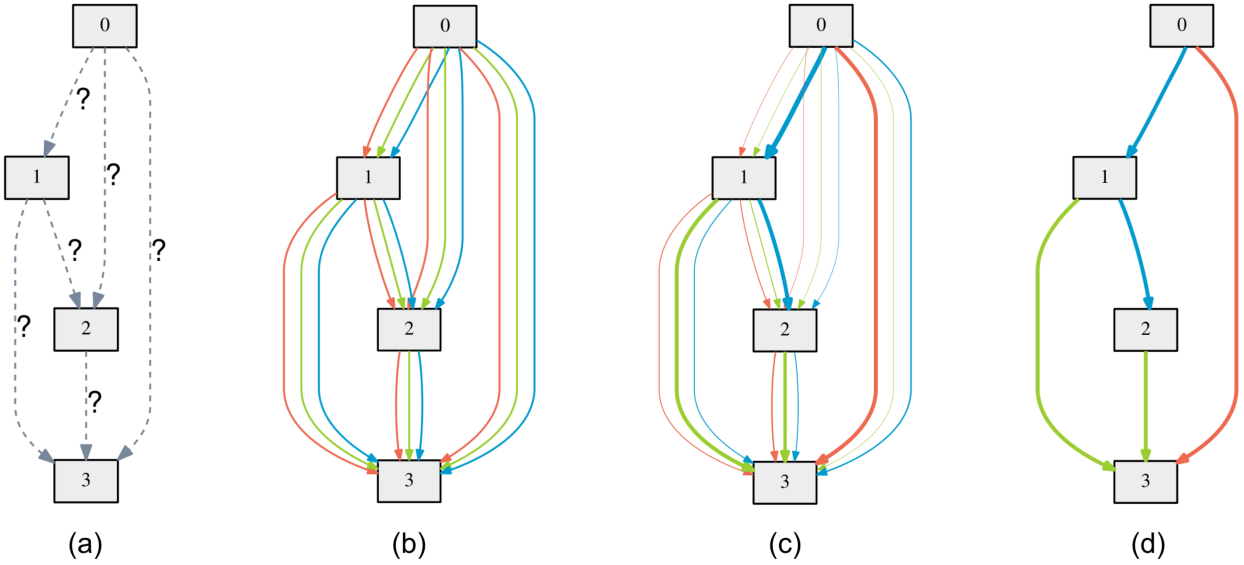
In the last year, a number of interesting results in differentiable architecture search started to emerge. DARTS (Liu et al., 2019) proposes to use gradient to search through the space of directed graphs. The authors first perform a continuous relaxation of the discrete graph, by reweighting the output of each potential edge by a hyperparameter, optimizing over the space of edges using gradient descent, then taking a softmax to discretize the output graph.

Solar-Lezma (2020) calls this latter approach, “program extraction”, where a network implicitly or explicitly parameterizes a function, which after training, can be decoded into a symbolic expression. This perspective also aligns with Ian Goodfellow’s notion of deep networks as performing computation, where each layer represents a residual step in a parallel program:
"Can neural networks be made to reason?" Conversation with Ian Goodfellow (@goodfellow_ian). Full version: https://t.co/3MYC8jWjwl pic.twitter.com/tGcDwgZPA1
— Lex Fridman (@lexfridman) May 20, 2019
A less charitable interpretation is that Goodfellow is simply using a metaphor to explain deep learning to lay audience, but I prefer to think he is communicating something deeper about the role of recurrent nonlinear function approximators as computational primitives, where adding depth effectively increases serial processing capacity and layer width increases bandwidth. There may be an interesting connection between this idea and arithmetic circuit complexity (Klivans and Shpilka, 2003).
Roadmap
Much work lies ahead for the interested reader. Before we can claim to have a unification of graph linear algebra and computer science, at least three technical hurdles will need to be cleared. First is theoretical: we must show that binary matrix mutiplication is Turing-equivalent. Second, we must show a proof-of-concept via binary recompilation. Third, we must develop a robust toolchain for compiling and introspecting a wide variety of graph programs.
While it would be sufficient to prove boolean matrix multiplication corresponds to Peano Arithmetic, a constructive proof taking physics into consideration is needed. Given some universal language \(\mathcal L\), and a program implementing a boolean vector function \(\mathcal V: \mathbb B^i \rightarrow \mathbb B^o \in \mathcal L\), we must derive a transformation \(\mathcal T_\mathcal L: \mathcal V \rightarrow \mathcal M\), which maps \(\mathcal V\) to a boolean matrix function \(\mathcal M: \mathbb B^{j \times k} \times \mathbb B^{l\times m}\), while preserving asymptotic complexity \(\mathcal O(\mathcal M) \lt \mathcal O(\mathcal V)\), i.e. which is no worse than a constant factor in space or time. Clearly, the identity function \(\mathcal I(\mathcal V)\) is a valid candidate for \(\mathcal T_{\mathcal L}\). But as recent GPGPU research has shown, we can do much better.
n.b. Not saying anything about the workload, just the architecture - Software 1.0 may still be the dominant paradigm. I'm saying there is a binary translation from load/store/jump/branch instructions to sparse BLAS primitives which imposes no constraints on the programming model.
— breandan (@breandan) July 1, 2020
The second major hurdle to graph computation is developing a binary recompiler which translates programs into optimized BLAS instructions. The resulting program will eventually need to demonstrate performant execution across a variety of heterogenously-typed programs, e.g. Int, Float16, Float32, and physical SIMD devices. Developing the infrastructure for such a recompiler will be a major engineering undertaking in the next two decades as the world transitions to graph computing. Program induction will likely be a key step to accelerating these graphs on physical hardware.
The third and final hurdle is to develop a robust compiler toolchain for graph computation. At some point, users will be able to feed a short program into a source-to-source transpiler and have the program slightly rewritten with semantics preserving guarantees. This will require progress in abstract interpretation, programming tools, runtime instrumentation, as well as shape-safe libraries and frameworks. Ultimately, we hypothesize users will adopt a more declarative programming style with resource-aware and type-directed constraints. This step will require fundamental progress in program induction and consume the better half of the next century to fully realize.
References
- Graph Representation Learning (Hamilton, 2020)
- Graph Algorithms in the Language of Linear Algebra (Kepner & Gilbert, 2011)
- Analysis of Boolean Functions (O’Donnell, 2014)
- Spectral and Algebraic Graph Theory (Spielman, 2019)
- GraphBLAS Mathematics (Kepner, 2017)
- Term Rewriting and All That (Baader & Nipkow, 1998)
- Representation of Events in Nerve Nets and Finite Automata (Kleene, 1951)
- A Class of Models with the Potential to Represent Fundamental Physics (Wolfram, 2020)